6.5. Screw Primitives

6.5.1. Motion Model

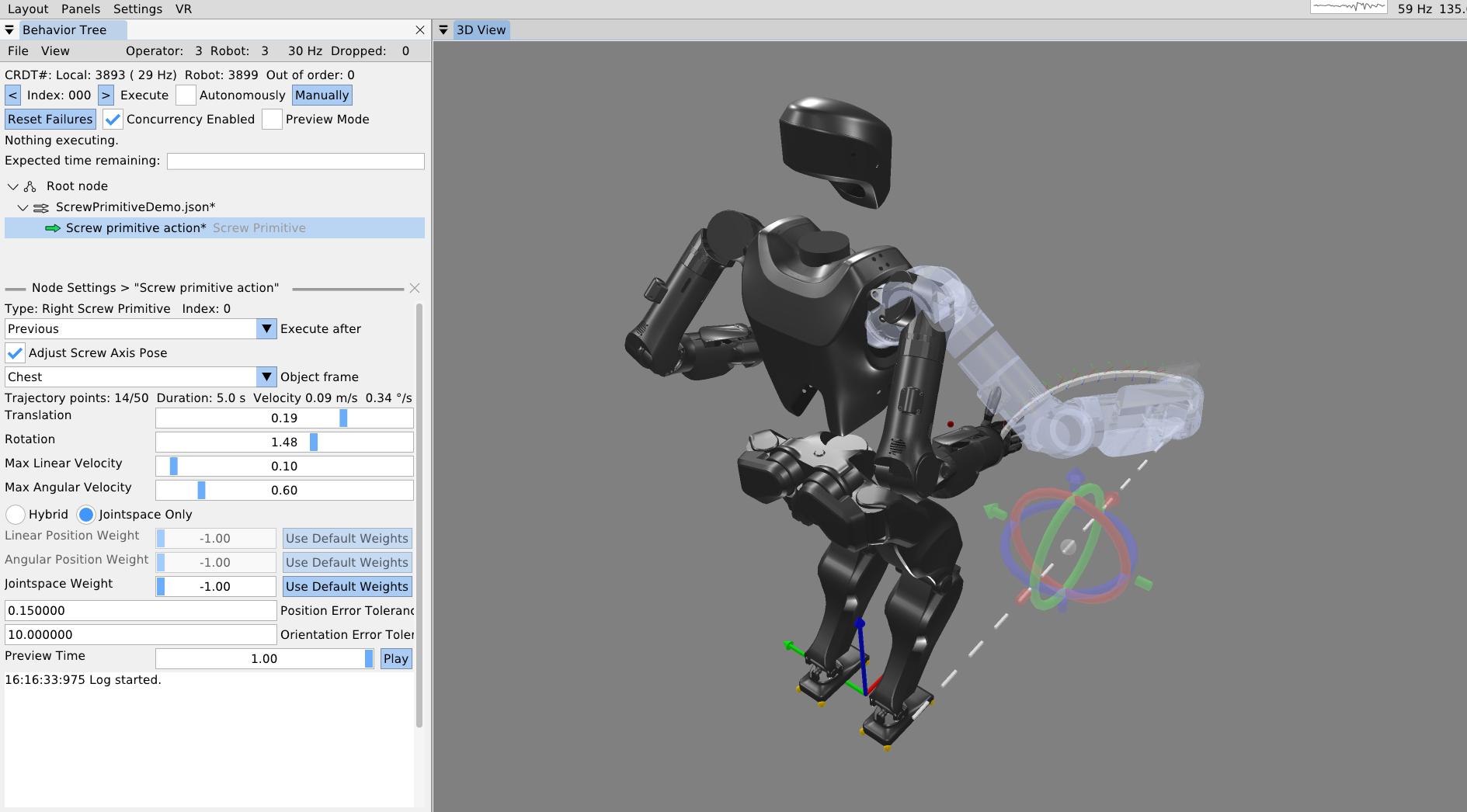
Figure 6.18 shows a screw primitive action being authored. Our screw primitive action is inspired by Pettinger’s 2022 paper  [14] but differs in implementation.

Our screw primitive action is defined relative to a user-defined screw reference frame, where the axis of the screw is strictly aligned with the local x-axis ($\hat{\mathbf{x}}$). The motion is parameterized by a total axial translation $\Delta x$ and a total rotation $\Delta \theta$. Figure 6.18 illustrates one parameterization for reference and the reference video shows varied parameterizations.

Let the initial position of the end-effector in the screw frame be $\mathbf{p}_0 = [x_0, y_0, z_0]^T$. The radial distance $r$ from the screw axis to the end-effector is calculated by projecting the position onto the y-z plane:

To compute motion bounds, the total Euclidean distance traversed by the end-effector, $D$, combines both the axial displacement and the tangential arc length:

The trajectory duration is determined by enforcing maximum velocity limits. Given a maximum linear velocity $v_{max}$ and maximum angular velocity $\omega_{max}$, the base duration $T_{base}$ required to complete the motion is dominated by the most restrictive bound:

The trajectory is discretized into $N$ waypoints (where $N$ is limited by the system’s trajectory buffer size), yielding $N-1$ segments. The nominal duration of a single segment is:

To account for smooth acceleration and deceleration without requiring complex spline generation, the implementation applies a temporal boundary condition: the duration of the first and last trajectory segments is doubled (i.e., $2\delta t$), while all intermediate segments retain duration $\delta t$. Consequently, the total movement duration expands to $T = T_{base} + 2\delta t$.

6.5.2. Trajectory Construction

The trajectory maintains constant base velocities throughout the central portion of the motion. The scalar velocities are derived from the base duration:

• Axial velocity: $v_a = \frac{\Delta x}{T_{base}}$

• Tangential velocity: $v_t = \frac{r \Delta \theta}{T_{base}}$

• Rotational velocity: $\omega_x = \frac{\Delta \theta}{T_{base}}$

At any intermediate waypoint $i$, let the current position of the end-effector in the screw frame be $\mathbf{p}_i = [x_i, y_i, z_i]^T$. The purely radial vector is $\mathbf{r}_{\perp, i} = [0, y_i, z_i]^T$.

The unit tangent vector $\mathbf{u}_{t,i}$ describing the instantaneous direction of rotation is found via the cross product of the screw axis and the radial vector:

The spatial velocity commands at waypoint $i$, expressed in the local screw frame, are formulated as:

Note that for the initial ($t=0$) and final ($t=T$) waypoints, the spatial velocities are strictly clamped to zero.

The rigid-body poses are iteratively generated by applying incremental transformations in the screw frame. For $K$ total segments (determined by spatial resolution limits), the incremental roll rotation $\delta \theta = \Delta \theta / K$ and translation $\delta x = \Delta x / K$ are calculated.

The pose of the end-effector at step $k$, denoted as $\mathbf{T}_k \in SE(3)$, is generated by prepending the incremental transformation to the previous pose:

This sequence of generated poses and spatial velocities is finally fed into an inverse kinematics solver to compute the joint-space trajectories.

6.5.3. Tuning and Preview

As seen in Figure 6.18, the total axial translation, total rotation, max linear velocity, and max angular velocity can be specified using sliders. The 3D trajectory visualization is updated in real time as the user drags these sliders to help dial in the motion. As with the single pose trajectory arm action, the screw primitive has settings for the position and orientation tolerance. If the final goal pose is not reached within these tolerances, the action fails.

In order to provide a rich intuition about the motion, there is also a motion preview slider for the screw primitive. The slider may be dragged manually or played back at real time speed in a loop. The arm is blue when the IK solution is good and red when it is bad. The behavior author should strive to keep it blue throughout the motion.

References cited on this page

[14] A. Pettinger, F. Alambeigi, and M. Pryor, “A versatile affordance modeling framework using screw primitives to increase autonomy during manipulation contact tasks,” IEEE Robotics and Automation Letters, vol. 7, no. 3, pp. 7224–7231, 2022, doi: 10.1109/LRA.2022.3181732.