6.4. Concurrent Actions Example
6.4.1. Behavior Timeline
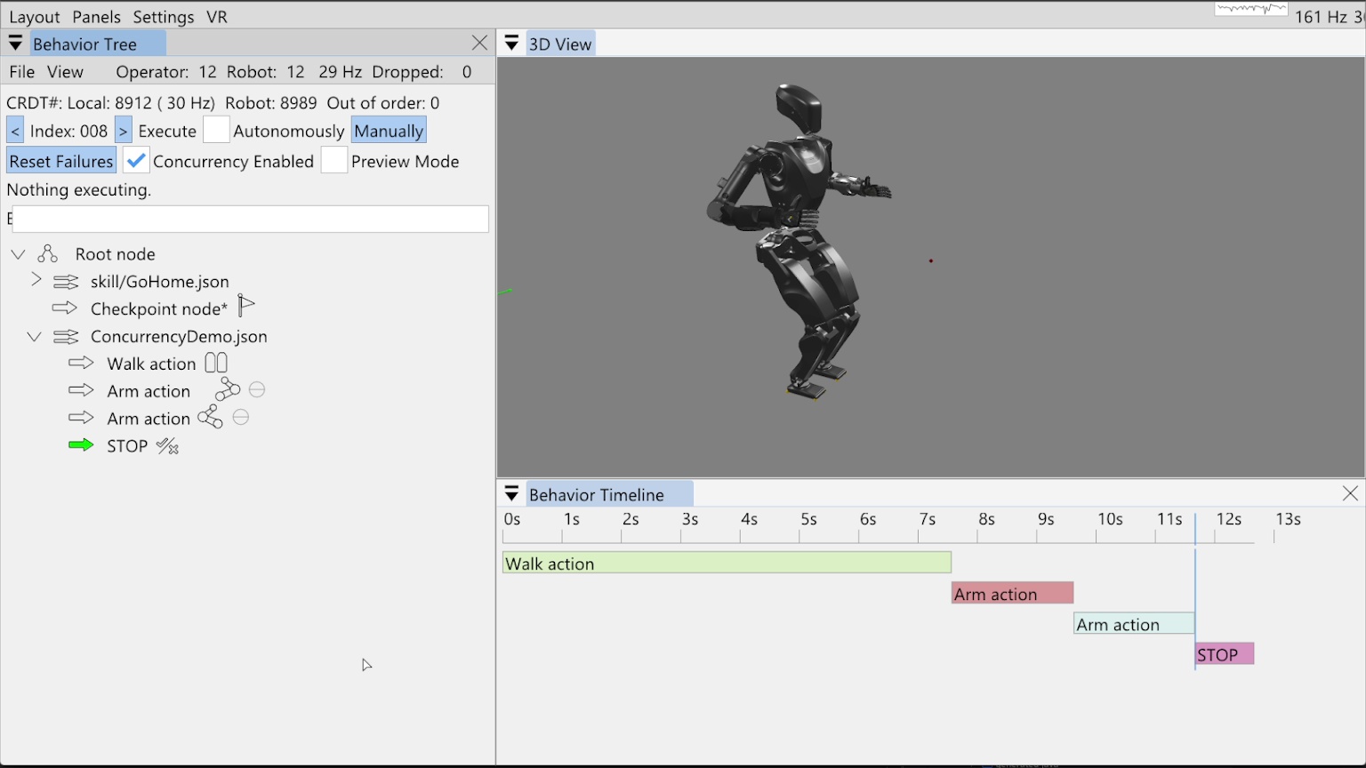
In this example, we’ll show how we can schedule arm motions while walking using our concurrent action layering system. Figure 6.14 shows a behavior we have already built and run as the non-concurrent starting place. In this tree, we have added the pre-existing “Go Home” skill from a file, which allows us to reset the robot to the home configuration. This home configuration has the arms down by the sides in a natural position. Then there is a checkpoint node and a savable concurrency demo behavior, with a walk action followed by two arm actions and an always failing “STOP” condition.
Our behavior timeline feature is presented in the bottom right of Figure 6.14. It is a rendering of an action sequence over time meant to help with understanding the timing and concurrency of behavior actions. Here, it shows the tree as executed with each node running sequentially.
6.4.2. “Execute After” Layering Mechanism
Concurrent action layering is implemented simply through an “Execute after” field in each action. It is selectable via a drop-down menu in the node settings, which offers every prior node as an option. By default this field is set to “Previous”, which is a dynamic reference to whatever node is immediately before. A dynamic “Beginning” reference is also available, which points to before the root node, though it may be removed because it is functionally the same as pointing to the ever-present root node.
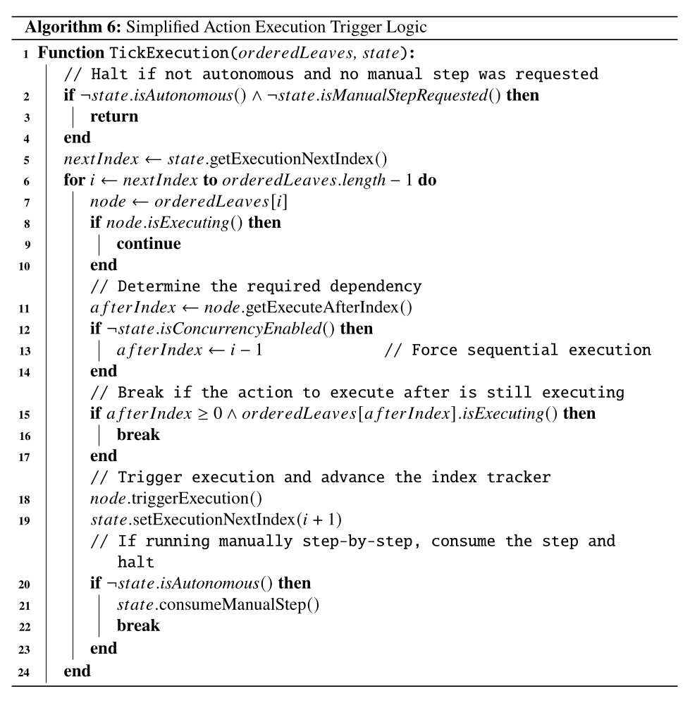
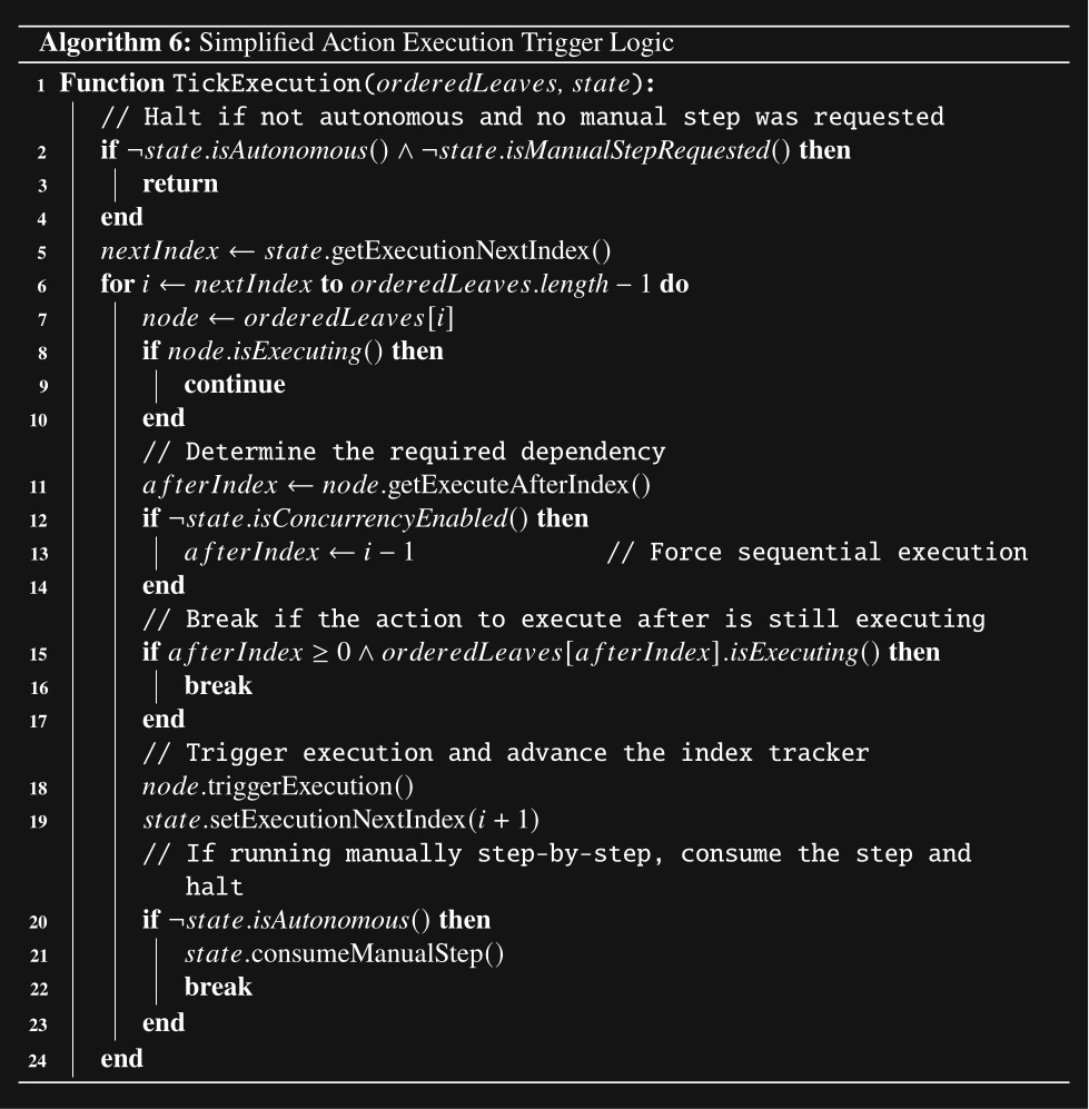
When the behavior is running in autonomous mode, it triggers action execution in order. When deciding whether to trigger execution of the next one, it first checks the referenced node to execute after. If the node to execute after is currently executing, the next node is not triggered. Importantly, action execution does not wait for any nodes that may be in between the “execute after” node and itself. This is important for scheduling concurrent actions freely.
The full algorithm is more complicated because the behavior can also be run step-by-step by clicking the “Manually” button. There is also a checkbox for disabling concurrency in the user interface, which effectively treats all “Execute after” fields as “Previous”. Further complexity is added to handle the fallback node’s try and catch mechanism. We present pseudocode in Algorithm 6 without the fallback part.
6.4.3. Wait Nodes and Dependencies
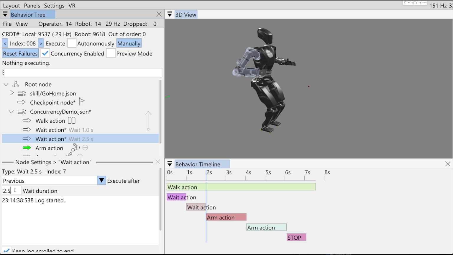
Our example behavior in Figure 6.14 starts out as a non-concurrent sequence of a short walk and two arm motions. Now we’ll change it so the arm motions are scheduled during the walk. In Figure 6.15, we add two wait actions, one for 1 second and one for 2.5 seconds. These waits are used to schedule the arm motions. We’ll move the right arm 1 second into the walk and the left arm 2.5 seconds into the walk.
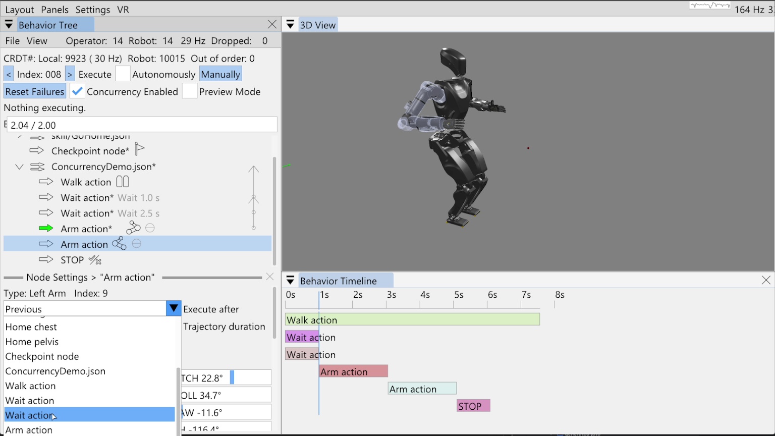
The wait actions need to execute with the walk action, not after it. To accomplish this, we set the execute after fields of the wait actions to the “ConcurrencyDemo.json” sequence node. The sequence node is never executing, but pointing to it achieves the effect that the wait actions always start with the walk action. This method also keeps the sequence logic self contained and reusable, as opposed to referencing a specific node earlier than the sequence node. We then set the execute after field of the right arm action to the first wait action and the execute after field of the left arm action to the second wait action. In Figure 6.16, we show setting the execute after field of the second arm action to the second wait action.
The figure also shows the execute after pointers as arrows on the right side of the tree view that point up from the defining action to the dependency action. You can see four such arrows that overlap. When the mouse hovers over a node, the corresponding arrow bolds to make it easy to verify dependencies when they are partially overlapping. At this point in time, the timeline view is updated to show the general structure of the new behavior configuration. In this prototype implementation of the timeline view, all wait actions are rendered as 1 second long. When we run the behavior, the timeline is redrawn with the actual timings. We will do that now.
6.4.4. Concurrent Result
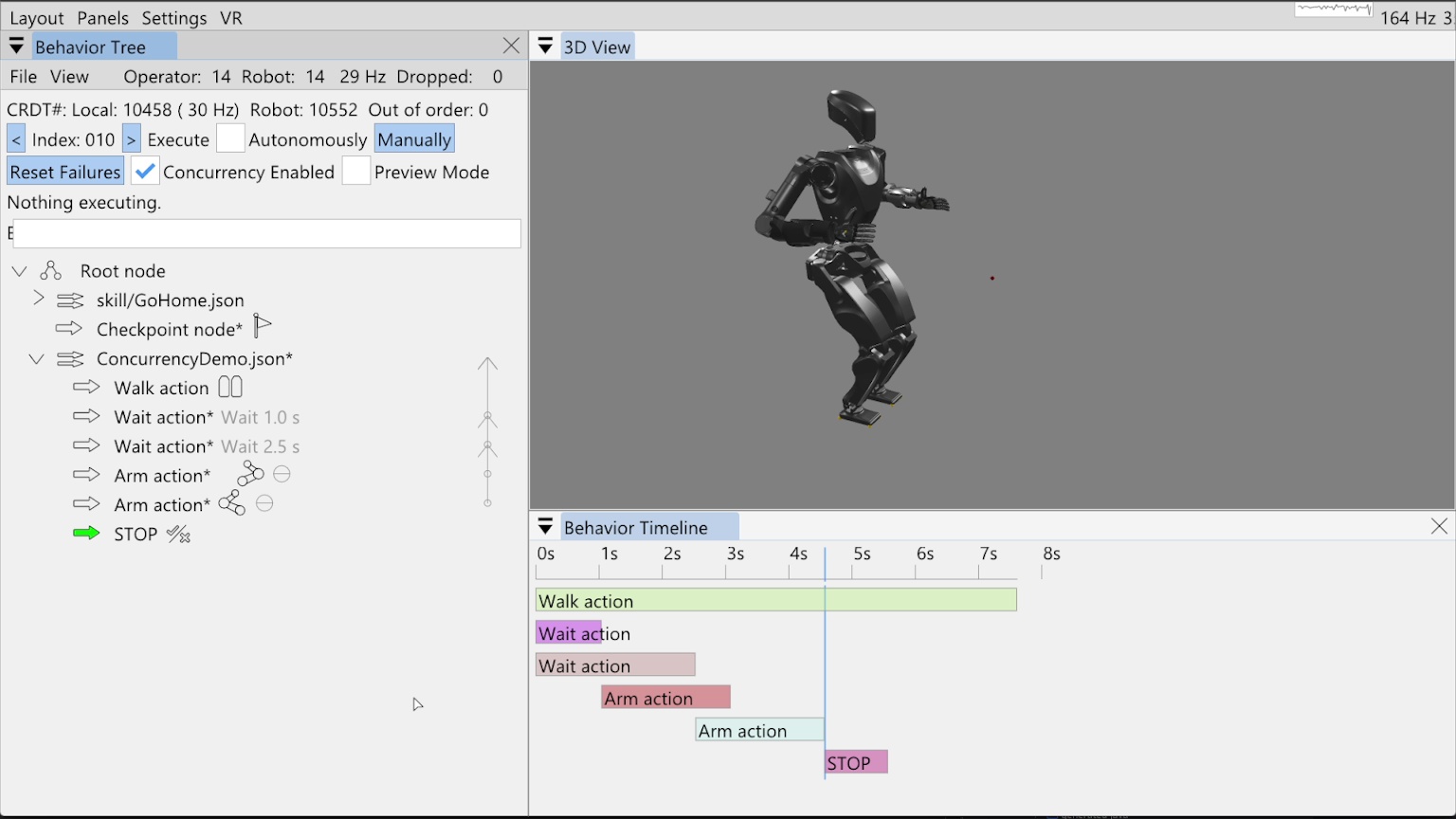
In Figure 6.17, we show the result of executing our now concurrent behavior. The timeline has been updated to reflect the actual action start and stop times of the simulated behavior execution. As seen by comparing this timeline to the original, the behavior duration went from 11.7 seconds to 7.6 seconds, illustrating how this method can be used to speed up behaviors.